Skydips and determination of the forward efficiency

In a skydip, the atmospheric emission, as seen by the receiver ( ), is measured at equally spaced airmass ( ). is a combination of the atmospheric emission and of losses

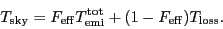$$\ensuremath{T_\ensuremath{\mathrm{sky}}\ifthenelse{\equal{}... ...m{loss}}\ifthenelse{\equal{}{}}{}{^\ensuremath{\mathrm{}}}}.$$ (7)

And the atmospheric emission is the sum of the atmospheric emission in both receiver bands

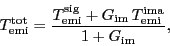$$\ensuremath{T_\ensuremath{\mathrm{emi}}\ifthenelse{\equal{t... ...\mathrm{ima}}}}}{1+\ensuremath{G_\ensuremath{\mathrm{im}}}},$$ (8)

each contribution computed from an equivalent atmospheric temperature and opacity $\tau$

$$\ensuremath{T_\ensuremath{\mathrm{emi}}\ifthenelse{\equal{s... ...{ima}{}}{}{_\ensuremath{\mathrm{ima}}}} \right) } \right\}}.$$ (9)

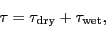
The zenith opacity can be written as a combination of a dry and wet components

$$\tau = \ensuremath{\tau\ifthenelse{\equal{dry}{}}{}{_\ensur... ...\tau\ifthenelse{\equal{wet}{}}{}{_\ensuremath{\mathrm{wet}}}},$$ (10)

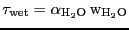
where is the opacity due to the permanent components of the atmosphere (mainly oxygen) and is proportional to the varying amount of water vapor amount ( ) in the atmosphere: $\ensuremath{\tau\ifthenelse{\equal{wet}{}}{}{_\ensuremath{\mathrm{wet}}}}= \ensuremath{\mathrm{\alpha_{H_2O}}}\,\ensuremath{\mathrm{w_{H_2O}}}$

Assuming that and are independent of the elevation and that and are correctly modeled by an atmospheric model, we obtain that is a function of , , , and the airmass ( ). If and are assumed to be measured by other means, then and can be fitted through the measured couples ( , ).